Advanced Higher Mathematics
Topics in this section
Review of Higher, Limits, Differentiation from 1st Principles, Continuity and Differentiability, Chain Rule, Product Rule, Quotient Rule. Derivatives of sec x, cosec x, tan x, cot x, Derivatives of exponential and logarithmic functions, Higher Derivatives, Inverse functions, Derivatives and graphs of inverse trigonometric functions. Chain Rule and product Rule applies to Inverse Trigonometric functions. Implicit Differentiation, Logarithmic Differentiation, Parametric Differentiation. Some applications of Differentiation and Exam style questions will feature where appropriate.
Review of Higher Differentiation
What you will learn:
In this lesson we will recap and review the Higher content of Differential Calculus.
We have put all of the Differential Calculus together in this chapter to make the topics easy to find.
Your school may present the material in a different order, or some material may be left until later in the course.
We have also put all of the Applications of Differentiation and Integration together in a separate Chapter 5 - Applications of Calculus, which follows on after Chapter 4 - Integration
In this way you should be able to locate the topic that you want, fairly easily.
You will find it useful to work through the examples using pencil and paper; and then to try to recreate them yourself.

Differentiation
At Higher we looked at Differentiation as a tool to extend our mathematical expertise.
We shall look back at some of the topics above but not all, as we shall be revisiting them during this chapter. The aim is to give a quick refresher of the Higher course prior to extending this knowledge with Advanced Higher.
At Advanced Higher we will look at differentiating more challenging functions as well as extending the types of function that we can differentiate. We will also look at how we can apply these new skills.
We will now briefly review the Higher content which will be a pre-requisite to this chapter
The Limit Formula
Given a function $y = f(x)$, and two points $P$ and $Q$ on the graph with x-coordinates $x$ and $x\ + \ h$ respectively and corresponding y-coordinates $f(x)$ and $f(x+h)$ as shown in the diagram below
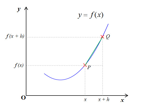
Let $PQ$ be a chord joining the points $P$ and $Q$ on the graph.
The gradient of the chord $PQ$ is given by:
(rise over run - or change in y divided by change in x)$$
m_{PQ} \;\; = \;\; \frac{y_Q - y_P}{x_Q-x_P} \\[18pt]
\implies \quad m_{PQ} \;\; = \;\; \frac{f(x+h) - f(x)}{(x+h) - x} \;\; = \;\; \frac{f(x+h) - f(x)}{h}
$$
If we allow point $Q$ to move towards point $P$ i.e. allow $h$ to get smaller and smaller until it shrinks towards zero,
Note that we say that $h$ tends to zero since we cannot divide by 0.
then the gradient of the chord $PQ$ will tend towards the gradient of the tangent at point $P$.
We write this as: 'the limit as $Q$ tends to $P$ ⇒ the gradient of PQ tends to the gradient of the tangent at $P$.
In mathematical notation which is much more concise:$$ \lim_{Q \to P}\ m_{PQ} \;\; = \;\; \lim_{h \to 0} \frac{f(x+h) - f(x)}{h} $$
We denote this limit which is the gradient of the tangent at $P$ by $f'(x)$.
So we have:$$ f'(x) \;\; = \;\; \lim_{h \to 0} \frac{f(x+h) - f(x)}{h} $$
The limit $f'(x)$ is known as the derivative of the function $f(x)$, since it is derived from $f(x)$. The process is known as differentiation and is the basis of the whole field of mathematics known as Differential Calculus.
The numerical value of this derivative at the point $x = a$ is the numerical value of the gradient of the tangent to the curve at the point $x = a$ which we write as: $$ f'(a) \;\; = \;\; \lim_{h \to 0} \frac{f(a+h) - f(a)}{h} $$
Let's look at a simple example to illustrate this:
Example:
Use the limit formula to find the derived function (the derivative) of $f(x) = x^2$ and find the gradient of the tangent to the curve at the point $x = 3$.
$$ f'(x) \;\; = \;\; \lim_{h \to 0} \frac{f(x+h) - f(x)}{h} \quad \text{and} \quad f(x) = x^2 \\[18pt] \implies \quad f'(x) \;\; = \;\; \lim_{h \to 0} \frac{(x+h)^2 - x^2}{h}\\[18pt] \implies \quad f'(x) \;\; = \;\; \lim_{h \to 0} \frac{x^2 + 2xh + h^2 - x^2}{h}\\[18pt] \implies \quad f'(x) \;\; = \;\; \lim_{h \to 0} \frac{2xh + h^2 }{h} $$ Dividing by $h$ we get $$ \implies \quad f'(x) \;\; = \;\; \lim_{h \to 0} ( 2x+h )\\[18pt] \implies \quad f'(x) \;\; = \;\; 2x $$ Hence at the point where $x=3$, the gradient of the curve is: $$ f'(3) \;\; = \;\; 2(3) \;\; = 6 $$
We can extend this to find the equation of the tangent to the curve at the point where $x = 3$.
We know that the gradient at the point where $\ x = 3\ $ is the gradient of the tangent at that point, i.e. $\ m = 6\ $
When $\ x = 3\ $, the value of $\ y\ $ is $\ x^2\ $ and so the coordinates of this point are $\left( 3,\ 9\right)$
Now we use the formula for the equation of a line using the point $\ \left(3,\ 9 \right)\ $ and the gradient $\ m = 6\ $. $$ y - b = m(x - a)\\[8pt] y - 9 = 6(x - 3)\\[8pt] y - 9 = 6x - 18\\[8pt] y = 6x - 9 $$
So the equation of the tangent to the curve $\ y = x^2\ $ at the point
where $\ x = 3\ $ is $\ y = 6x - 9$.
This process is called Differentiation from 1st Principles. It is an unwieldy process at times but it is essential for deriving rules which we can use to make the process of Differentiation much simpler and faster.
We shall use practise using differentiation from 1st principles in the next chapter.
The notation used above, $f'(x)$ is known as Newton's notation.
Sir Isaac Newton developed the theory of Calculus at the same time as Gottfried Wilhelm Leibniz, a German Mathematician in the 17th century.
We will now look at Leibniz' notation.
The Limit Formula in Leibniz' notation
Given a function $y = f(x)$, and two points $P$ and $Q$ on the graph with x-coordinates $x$ and $x\ + \ \Delta x$ respectively and corresponding y-coordinates $y$ and $y+\Delta y$ as shown in the diagram below
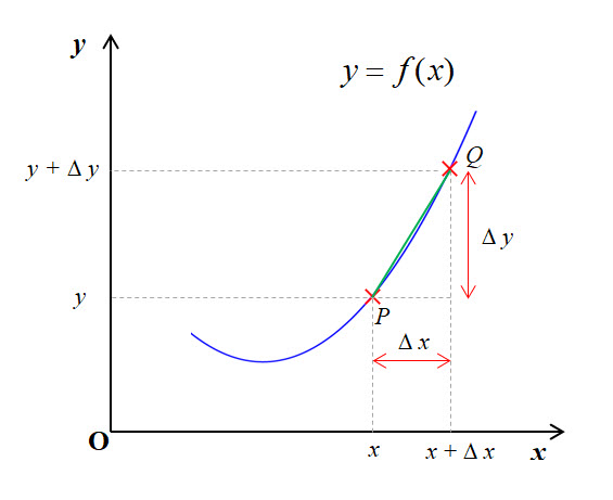
Let $PQ$ be a chord joining the points $P$ and $Q$ on the graph.
The gradient of the chord $PQ$ is given by:
(rise over run - or change in y divided by change in x)$$
m_{PQ} \;\; = \;\; \frac{\Delta y}{\Delta x} \\[18pt]
$$
If we allow point $Q$ to move towards point $P$ i.e. allow $\Delta x$ to get smaller and smaller until it shrinks towards zero.
Note that we say that $\Delta x$ tends to zero since we cannot divide by 0.
Then the gradient of the chord $PQ$ will tend towards the gradient of the tangent at point $P$.
We write this as: 'the limit as $Q$ tends to $P$ ⇒ the gradient of PQ tends to the gradient of the tangent at $P$.
In mathematical notation which is much more concise:$$ \lim_{Q \to P}\ m_{PQ} \;\; = \;\; \lim_{\Delta x \to 0} \frac{\Delta y}{\Delta x} $$
We denote this limit which is the gradient of the tangent at $P$ by $\Large \frac{dy}{dx}$.
So we have:$$ \frac{dy}{dx} \;\; = \;\; \lim_{\Delta x \to 0} \frac{\Delta y}{\Delta x} $$
The limit $ \Large \frac{dy}{dx}$ is known as the derivative of the function $f(x)$, since it is derived from $f(x)$.
Other notations used for the derivative are:$$ f'(x), \;\; y', \;\; y'(x), \;\; \frac{dy}{dx}, \;\; \frac{df}{dx}, \;\; \frac{d}{dx}f(x) $$as well as using other variables such as$$ g'(x), \;\; \frac{dy}{dt},\;\; \frac{dg}{dt} \;\; etc. $$In all cases these are the derivative of the function, with respect to the variable specified.
We shall see many different variables and function names used in this course and in this chapter.
The numerical value of this derivative at the point $x = a$ is the numerical value of the gradient of the tangent to the curve at the point $\ x = a\ $ which is often written as: $$ {\left. {\frac{{dy}}{{dx}}} \right|_{\large x = a}} $$
Again let's look at a simple example to illustrate this:
Example:
Use the limit formula with Leibniz' notation to find the derived function (the derivative) of $f(x) = x^2$ and find the gradient of the tangent to the curve at the point $x = 4$.
$$ \frac{dy}{dx} \;\; = \;\; \lim_{\Delta x \to 0} \frac{\Delta y}{\Delta x} \;\; = \;\; \frac{(y + \Delta y) - y}{\Delta x} \quad \text{and} \quad y = x^2 \\[18pt] \implies \quad \frac{dy}{dx} \;\; = \;\; \lim_{\Delta x \to 0} \frac{(x+\Delta x)^2 - x^2}{\Delta x}\\[18pt] \implies \quad \frac{dy}{dx} \;\; = \;\; \lim_{\Delta x \to 0} \frac{x^2 + 2x \Delta x + {(\Delta x)}^2 - x^2}{\Delta x}\\[18pt] \implies \quad \frac{dy}{dx} \;\; = \;\; \lim_{\Delta x \to 0} \frac{2x\Delta x + {(\Delta x)}^2 }{\Delta x} $$ Dividing by $\Delta x$ we get $$ \implies \quad \frac{dy}{dx} \;\; = \;\; \lim_{\Delta x \to 0} ( 2x+\Delta x )\\[18pt] \implies \quad \frac{dy}{dx} \;\; = \;\; 2x $$ Hence at the point where $x=4$, the gradient of the tangent to the curve is: $$ {\left. {\frac{{dy}}{{dx}}} \right|_{\large x = 4}} \;\; = \;\; 2(4) \;\; = \;\; 8 $$
It is your choice which notation to use, sometimes one may be appropriate than the other. When differentiating from 1st Principles, then the Newton notation is probably easier to follow.
As a general rule if your function is in the form $\ y =\ ...\ $ then use Leibniz' notation. If the function is given in the form $\ f(x) =\ ...\ $ then use Newton's notation. However, it really is up to you.
Some Reminders
Derivatives of basic algebraic functions of the form $ax^n$
$$ y = ax^n \quad \implies \quad \frac{dy}{dx} \;\; = \ \ n\ ax^{n-1} $$
Variable in the denominator
Always write the function in straight line form before differentiating. $$ f(x) = \frac{3}{x^2} \quad \implies \quad f(x) = 3x^{-2} \\[18pt] \implies \quad f'(x) = (-2) \times 3 x^{-3} \quad \implies \quad f'(x) = -6x^{-3}\\[18pt] \implies \quad f'(x) = -\frac{6}{x^3} $$
Sums and Differences
Differentiate term by term: $$ f(x) = a\ g(x) \; \pm \; b\ h(x) \quad \implies \quad f'(x) = a\ g'(x) \; \pm \; b\ h'(x)\\[12pt] \text{e.g.} \ \ f(x) = 3x^5 - 4x^2 \quad \implies \quad f'(x) = 15x^4 - 8x $$
Function is a simple fraction
Split into separate fractions: $$ f(x) = \frac{5x^3 + 4x^2}{x} \quad \implies \quad f(x) = \frac{5x^3}{x} + \frac{4x^2}{x} \\[18pt] \implies \quad f(x) = 5x^2 + 4x \quad \implies \quad f'(x) = 10x + 4 $$
Linear and constant functions
$$ y \;= \; k\thinspace x \quad \implies \quad \frac{dy}{dx} \; = \; k \\[18pt] y \;= \; k \quad \implies \quad \frac{dy}{dx} \; = \; 0 $$
Continuity and Differentiability
For a function to be differentiable, at the point $x = a$:
Returning to our diagram, it has to be possible for the chord to move down the curve to form the tangent at the point.
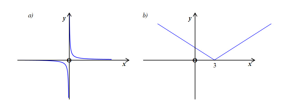
In diagram a), the function is not differentiable at the point $x=0$ since the function is undefined at $x=0$ and neither is the function continuous at that point.
In diagram b), the function is not differentiable at the point $x=3$ since although the function is defined at that point and continuous, the left hand and right hand limits are not the same. The left hand limit is negative and the right hand limit is positive.
Continuity and differentiability will be covered in more detail in Chapter 6 - Properties of Functions
Trigonometric Functions
When working with trigonometric functions, you should work in radians. The reason for that is the derivative we are familiar with is the result of taking the limit when the angle is in radians.
We could work with degrees, but the limit would have a different value:$$ \frac{d}{dx} \ sin (x ^{\circ}) \; = \; \frac{\pi}{180} cos (x ^{\circ})$$ which is unwieldly, to say the least. So make sure you work in radians.
Trigonometric Derivatives when working in Radians
$$ y \; = \; sin (ax) \quad \implies \quad \frac{dy}{dx}\; = \; a\ cos\ (ax)\\[18pt] y \; = \; cos (ax) \quad \implies \quad \frac{dy}{dx}\; = \; -a\ sin\ (ax) $$
Chain Rule
Given that:$$ \eqalign{ &y \; = \; f\left( g(x) \right)\quad \quad \quad (1) \hspace{10cm}\\[12pt] &\text{Let }\ u \; = \; g(x) \quad \quad \\[12pt] &\text{Substituting for }\ g(x)\ \text{ in (1) } \;\; \implies \;\; y \; = \; f(u) \quad \quad \\[12pt] &\text{So, differentiating with respect to }\ u \;\; \implies \;\;\frac{dy}{du} \; = \; \frac{df}{du} \quad \\[12pt] &\text{However, we want the derivative with respect to }\ x \\[12pt] &\text{So multiply by } \ \frac{du}{dx} \\[12pt] &\implies \;\;\frac{dy}{dx} \; = \; \frac{df}{du} \times \frac{du}{dx}\;\; = \;\; \frac{df}{dx} \;\; = \;\; f'(x)\\[12pt] } $$Putting it all together as a rule: $$ y \;\;= \;\; f(g(x)) \quad \implies \quad \frac{dy}{dx} \;\; = \;\; \frac{df}{dg} \times \frac{dg}{dx} $$We shall look at the Chain Rule in more detail, later in this chapter.
Let's do an example to clarify this:
Example:
Given that $y = \left( 5x^3 + 2x + 1\right)^3$, find the derivative $\Large \frac{dy}{dx}$
$$ y = \left( 5x^3 + 2x + 1\right)^3\\[12pt] \text{Let } \ u = 5x^3 + 2x + 1 \\[12pt] \text{then } \ y \;\; = \;\; u^3 \\[12pt] \text{So } \ \frac{dy}{du} \;\; = \;\; 3u^2 \\[12pt] \text{also } \ \frac{du}{dx} \;\; = \;\; 15x^2 + 2 \\[12pt] \text{Thus } \ \frac{dy}{dx} \;\; = \;\; \frac{dy}{du} \times \frac{du}{dx} \\[12pt] \implies \frac{dy}{dx} \;\; =\;\; 3\left( 5x^3 + 2x + 1 \right)^2 \ \left( 15x^2 + 2 \right) \\[12pt] $$We can actually do this much easier by considering the rule in terms of a bracket: $$ y \;\; = \;\; \left( .... \right)^n\\[12pt] \frac{dy}{dx} \;\; = \;\; n\ \left( .... \right)^{n-1} \times \frac{d}{dx} \ \left( .... \right)\\[12pt] $$The function inside the bracket $\ \left( .... \right)^n $ is called the essential function. We shall see how this works in more detail in a later lesson.
For example if we have $\ y = \left( 2x^3 - 5x^2+1 \right)^4\ $ then $\ 2x^3 - 5x^2 + 1\ $ is the essential function since this function is being raised to the power 4 and as the contents of the bracket, it will be differentiated, to form the multiplier in the derivative.
Let's do another example to illustrate this:
Example:
Given that $y = \left( 7x^2 + 2x + 3\right)^4$, find the derivative $\Large \frac{dy}{dx}$
The essential function is $\ 7x^2+2x+3$. $$ y = \left( 7x^2 + 2x + 3\right)^4\\[12pt] \frac{dy}{dx} \;\; = \;\; 4\left( .... \right)^3 \times \frac{d}{dx} \left( .... \right) \\[12pt] \color{darkgray}{\frac{dy}{dx} \;\; = \;\; 4\left( 7x^2 + 2x + 3 \right)^3 \times \frac{d}{dx} \left( 7x^2 + 2x + 3 \right)} \\[12pt] \implies \;\; \frac{dy}{dx} \;\; = \;\; 4\left( 7x^2 + 2x + 3 \right)^3 \left( 14x + 2 \right) $$As you can see, we can almost write this down doing the working mentally.
Chain Rule with Trigonometric Functions
In essence, this is applied in exactly the same way. Consider the following example, to which we will add extra explanation.
Example:
Given that $y = sin^3 (3x)$, find the derivative $\Large \frac{dy}{dx}$
The essential function here is: $sin\ 3x$
because we can write $\ y = sin^3 (3x) \ $ as:$\ \ y = \left( sin\ 3x \right)^3$
So by considering this as:$$ y = \left( sin\ 3x \right)^3\\[12pt] \implies \quad \frac{dy}{dx} \;\; = \;\; 3\left( sin \ 3x\right)^2 \times 3\ cos\ 3x\\[12pt] \implies \quad \frac{dy}{dx} \; = \; 9\ sin^2 \ 3x\ cos\ 3x $$Again, we can see how much benefit is obtained by using the bracket interpretation and identifying the essential function.
Stationary Points
We also used differentiation to find the stationary points on a curve. We used a table of signs to determine their nature, as to whether they were a maximum, a minimum or a point of inflexion.
Again, let's use a quick example to illustrate this as a refresher.
Example:
Find the coordinates of the turning points of the function $ y = x^3 -3x\ $ and determine their nature.
The first step is to differentiate the function: $$ y = x^3 -3x \\[12pt] \frac{dy}{dx} = 3x^2 - 3 $$ For a stationary point, the gradient $\ \Large \frac{dy}{dx} \normalsize = 0 $
Equating the derivative to $0$: $$ \frac{dy}{dx} = 0 \quad \implies \quad 3x^2 - 3 \; = \; 0\\[12pt] \implies \quad 3x^2 \;=\; 3 \\[12pt] \implies \quad x^2 \;=\; 1\\[12pt] \implies \quad x = 1 \ \text{ or } \ x = -1 $$ When $$\ x \; = \; 1 \quad \implies \quad y\; =\; 1^3 - 3(1) \quad = \quad -2 \\[12pt] \implies \;\; \text{S.P. at }\ \left(1,\ -2 \right)$$ When $$\ x \; = \; -1 \quad \implies \quad y\; =\; \left(-1\right)^3 - 3\left(-1\right) \quad = \quad 2 \\[12pt] \implies \;\; \text{S.P. at }\ \left(-1,\ 2 \right)$$
Determine the nature of the SPs by using the table of signs.
| $\scriptsize x=-2$ | $\scriptsize x=0$ | $\scriptsize x=2$ | |||
|---|---|---|---|---|---|
| $x$ | $\to$ | $-1$ | $\to$ | $1$ | $\to$ |
| $\large \frac{dy}{dx}$ | $+$ | $0$ | $-$ | $0$ | $+$ |
| Gradient | / | − | \ | − | / |
| Nature | maximum | minimum |
There is a maximum S.P. at $\ (-1,\ 2)$ and a minimum S.P. at $\ (1, \ -2 )$.
Note that the y-coordinates of $2$ and $-2$ are known as the stationary values of the function.
By looking at the table of signs, we can see that the function is:
increasing from $\ -\infty\ \lt x \lt -1 \ $
decreasing from $\ -1\ \lt x \lt 1 \ $
increasing again from $\ 1\ \lt x \lt \infty \ $
as we can confirm by looking at the graph below.
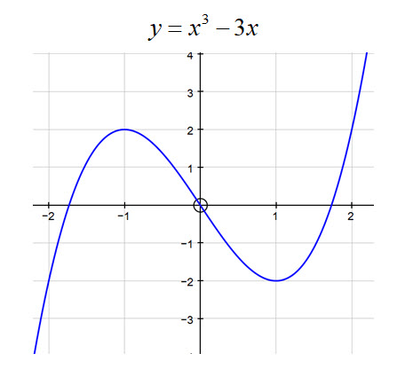
As we can deduce all of this information from the table of signs, it is a very powerful tool for helping us to sketch the graph of a function as we shall see later in this chapter.
You should be familiar with the limit formula and both Newton's and Leibniz' notation for the derivative.
You should be able to differentiate basic functions and use the chain rule.
You should be able to find stationary points, determine their nature and use them effectively.
You should understand fully the meaning of the derivative and how you can use it.
You have now briefly reviewed the content of Differentiation in the Higher course and should feel confident about moving on with the Advanced Higher material.
Go to the next topic in the side menu to learn more about Limits and Differentiating from 1st Principles.
Review of Higher Differentiation
Sorry we have no worked examples available yet for this topic.
Status Update
We will regularly update the status of the website here.
In view of the pandemic restrictions, we have decided to focus on Advanced Higher for the time being.
Consequently, we will just add the lessons to the site and add the worked examples, exercises and solutions as time permits.
We will add a video version of the lessons at a later date.
We have also amended the site code to show unselected tabs containing content with a light green background and without content with a light grey background, so you do not need to keep clicking on them to check if there is any new content.
19th August 2021 More Content will be posted soon.
Due to other commitments there is a constraint on time.
Apologies for any inconvenience.
3rd October 2021 More Content will be posted soon.
Due to other commitments there is a constraint on time.
Apologies for any inconvenience.
11th January 2022 Corrected error in National 5 Surds.
Example 2
14th April 2022 More Content will be posted soon.
Still as a result of other commitments there is a constraint on time.
Apologies for any inconvenience.
Currently working on:
Advanced Higher - Integration
Further Integration by Parts
Topics coming soon in this Chapter - Advanced Higher:
Areas between curves and the axes.
Volumes of Revolution.
Next Chapters - Advanced Higher
Applications of Calculus
Properties of Functions
Systems of Equations
If you spot any errors, typos or broken links,
or even if you just want to make a comment,
I would be pleased if you would contact me by email,
contact@maths4scotland.co.uk
Review of Higher Differentiation
Sorry we have no Exercise available yet for this topic.
Status Update
We will regularly update the status of the website here.
In view of the pandemic restrictions, we have decided to focus on Advanced Higher for the time being.
Consequently, we will just add the lessons to the site and add the worked examples, exercises and solutions as time permits.
We will add a video version of the lessons at a later date.
We have also amended the site code to show unselected tabs containing content with a light green background and without content with a light grey background, so you do not need to keep clicking on them to check if there is any new content.
19th August 2021 More Content will be posted soon.
Due to other commitments there is a constraint on time.
Apologies for any inconvenience.
3rd October 2021 More Content will be posted soon.
Due to other commitments there is a constraint on time.
Apologies for any inconvenience.
11th January 2022 Corrected error in National 5 Surds.
Example 2
14th April 2022 More Content will be posted soon.
Still as a result of other commitments there is a constraint on time.
Apologies for any inconvenience.
Currently working on:
Advanced Higher - Integration
Further Integration by Parts
Topics coming soon in this Chapter - Advanced Higher:
Areas between curves and the axes.
Volumes of Revolution.
Next Chapters - Advanced Higher
Applications of Calculus
Properties of Functions
Systems of Equations
If you spot any errors, typos or broken links,
or even if you just want to make a comment,
I would be pleased if you would contact me by email,
contact@maths4scotland.co.uk
Review of Higher Differentiation
Sorry we have no solutions available yet for this topic.
Status Update
We will regularly update the status of the website here.
In view of the pandemic restrictions, we have decided to focus on Advanced Higher for the time being.
Consequently, we will just add the lessons to the site and add the worked examples, exercises and solutions as time permits.
We will add a video version of the lessons at a later date.
We have also amended the site code to show unselected tabs containing content with a light green background and without content with a light grey background, so you do not need to keep clicking on them to check if there is any new content.
19th August 2021 More Content will be posted soon.
Due to other commitments there is a constraint on time.
Apologies for any inconvenience.
3rd October 2021 More Content will be posted soon.
Due to other commitments there is a constraint on time.
Apologies for any inconvenience.
11th January 2022 Corrected error in National 5 Surds.
Example 2
14th April 2022 More Content will be posted soon.
Still as a result of other commitments there is a constraint on time.
Apologies for any inconvenience.
Currently working on:
Advanced Higher - Integration
Further Integration by Parts
Topics coming soon in this Chapter - Advanced Higher:
Areas between curves and the axes.
Volumes of Revolution.
Next Chapters - Advanced Higher
Applications of Calculus
Properties of Functions
Systems of Equations
If you spot any errors, typos or broken links,
or even if you just want to make a comment,
I would be pleased if you would contact me by email,
contact@maths4scotland.co.uk